机器学习中交叉验证行为的可视化（scikit-learn）

机器学习中交叉验证行为的可视化（scikit-learn）

交叉验证（cross-validation）是一种用于评估机器学习模型性能的统计学方法。它通过将数据集划分为多个互不重叠的子集，然后利用其中一部分数据作为训练集，另一部分数据作为试集来训练和测试模型。这个过程会进行多次，每次使用不同的子集作为测试集，最终计算模型在不同测试集上的性能指标。交叉验证可以有效地评估模型的性能和泛化能力，避免模型在特定数据集上过度拟合或欠拟合的情况，同时也可以帮助选择最佳的模型超参数，如学习率、正则化参数、网络层数等。

为了验证交叉验证行为的正确性，我们可以对交叉验证过程中划分好的数据集进行可视化，来直观的对交叉验证进行观察。我们以scikit-learn实现的k-fold交叉验证为例，来实现对交叉验证行为的可视化。

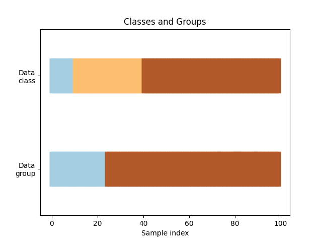
生成虚拟数据

首先我们需要生成一些虚拟的数据。这些数据用来模拟一个常见的机器学习分类任务的数据集，例如：一个三分类的疾病分类任务，三种类别的疾病分布在人群中，这个人群分为“男”、“女”两个“组”，三种类别的数据均匀的分布在两个组中。我们随机生成100个数据点，这个生成的数据集中有三个类别，这三个类别不均匀的分布在数据集中，但是均匀的分布在两个组中。

# 导入相关的包
import matplotlib.pyplot as plt
import numpy as np
from matplotlib.patches import Patch
from sklearn.model_selection import KFold

编写生成数据的函数generate_data()，其中n_points为生成的数据点个数，n_features为生成数据的特征数，n_groups为分组数，percentiles_classes为每种类别所占的比例。

def generate_data(n_points: int = 100,
                  n_features: int = 10,
                  n_groups: int = 2,
                  percentiles_classes: list[float] = None) -> tuple:
    if percentiles_classes is None:
        percentiles_classes = [0.1, 0.3, 0.6]
    X = np.random.randn(n_points, n_features)
    y = np.hstack(
        [[i] * int(100 * perc) for i, perc in enumerate(percentiles_classes)])
    group_prior = np.random.dirichlet([2] * n_groups)
    groups = np.repeat(np.arange(n_groups),
                       np.random.multinomial(n_points, group_prior))
    return X, y, groups

数据分组可视化

接下来，实现一个数据可视化的的函数visualize_data来帮助我们直观的观察到数据中的类别以及组的分布情况。

def visualize_data(classes: np.ndarray, 
                   groups: np.ndarray,
                   name: str = 'Classes and Groups') -> None:
    fig, ax = plt.subplots()
    ax.scatter(
        range(len(groups)),
        [0.5] * len(groups),
        c=groups,
        marker="_",
        lw=50,
        cmap=plt.cm.Paired,
    )
    ax.scatter(
        range(len(groups)),
        [3.5] * len(groups),
        c=classes,
        marker="_",
        lw=50,
        cmap=plt.cm.Paired,
    )
    ax.set(
        ylim=[-1, 5],
        yticks=[0.5, 3.5],
        yticklabels=["Data\ngroup", "Data\nclass"],
        xlabel="Sample index",
    )
    ax.set_title(name)
    plt.show()

通过调用上面的函数，我们可以观察到我们生成的数据的分组情况，三个类别与两个组并不是均匀的分布在整个数据集中：

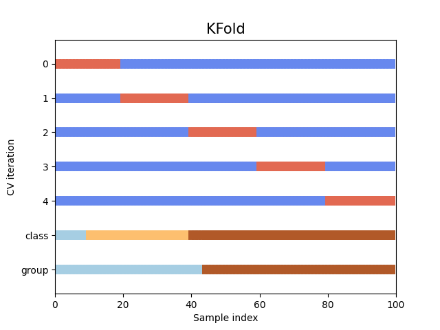
可视化交叉验证行为

接下来，我们定义一个函数来可视化交叉验证行为。该函数允许我们传入一个交叉验证的对象，并且对其所划分的测试机与验证集进行直观的展示。

def visualize_cv(cv, 
                 X: np.ndarray, 
                 y: np.ndarray, 
                 group: np.ndarray,
                 n_splits: int = 5, 
                 lw: int = 10) -> None:
    fig, ax = plt.subplots()
    use_groups = "Group" in type(cv).__name__
    groups = group if use_groups else None
    for ii, (tr, tt) in enumerate(cv.split(X=X, y=y, groups=groups)):
        indices = np.array([np.nan] * len(X))
        indices[tt] = 1
        indices[tr] = 0

        ax.scatter(
            range(len(indices)),
            [ii + 0.5] * len(indices),
            c=indices,
            marker="_",
            lw=lw,
            cmap=plt.cm.coolwarm,
            vmin=-0.2,
            vmax=1.2,
        )

        ax.scatter(
            range(len(X)),
            [ii + 1.5] * len(X),
            c=y, marker="_",
            lw=lw,
            cmap=plt.cm.Paired
        )

        ax.scatter(
            range(len(X)),
            [ii + 2.5] * len(X),
            c=group,
            marker="_",
            lw=lw,
            cmap=plt.cm.Paired
        )

    yticklabels = list(range(n_splits)) + ["class", "group"]
    ax.set(
        yticks=np.arange(n_splits + 2) + 0.5,
        yticklabels=yticklabels,
        xlabel="Sample index",
        ylabel="CV iteration",
        ylim=[n_splits + 2.2, -0.2],
        xlim=[0, 100],
    )
    ax.set_title("{}".format(type(cv).__name__), fontsize=15)
    plt.show()

cv = KFold(5)
visualize_cv(cv, X, y, groups, 5)

我们以一个5折交叉验证为例，5折交叉验证的cv对象会将原始数据集分成五个相等大小的子集（或折叠fold），其中四个子集用于训练模型，而剩下的一个子集用于测试模型。这个过程重复五次，每次选择不同的一个子集作为测试集，其余的作为训练集。最后，将五次的性能评估结果取平均值以得到最终评估结果。最终的可视化结果如下：

可以直观地看到，在默认情况下，KFold 交叉验证迭代器不考虑数据点类别或组。

通过这种方式，可以直观地让我们对包含多个类别与组的数据分布进行观察，同时以直观的方式观察交叉验证行为，方便我们对交叉验证行为的正确性进行初步的检验。